CTO: Resolution-Agnostic Neural Operators for Multi-Rate Sparse-View CT

Sparse-view Computed Tomography (CT) reconstructs images from a limited number of X-ray projections to reduce radiation and scanning time, which is an ill-posed inverse problem. Existing methods achieve high-fidelity reconstructions but overfit to a fixed acquisition setup, failing to generalize well across sampling rates. For example, convolutional neural networks (CNNs) use the same kernels across resolutions, leading to artifacts when data resolution changes. This is a critical limitation in clinical practice, where acquisition sampling settings vary across organs and diagnostic protocols.

We propose Computed Tomography neural Operator (CTO), the first neural operator (NO) framework for CT reconstruction. CTO extends learning from fixed discretized grids to continuous function space, enabling a single model to generalize across measurement sampling rates without retraining. We also propose new NO architectural designs for CT: (i) a dual-domain NO architecture in both sinogram and image spaces, capturing complementary spatial–frequency information, and (ii) rotation-equivariant DIScrete–COntinuous convolutions (DISCO) that exploit the rotational structure inherent in tomographic acquisition. Empirically, CTO outperforms CNNs (> 3.4dB PSNR gain) and other baselines in multi-resolution settings across multiple CT datasets. Compared to state-of-the-art diffusion methods, CTO has 500× faster inference with an average 3dB gain. CTO further demonstrates strong out-of-distribution robustness, maintaining gains under cross-dataset transfer and noisy sinogram conditions. Ablation studies also validate each design choice. CTO establishes neural operators as a principled and practical paradigm for flexible, discretization-agnostic CT reconstruction.

Index

Computed Tomography

CT is an imaging modality where an X-ray source and detector rotate around the patient, and along each angle we get a 1-D projection which is the line integral of attenuation. This is mathematically denoted by the Radon transform $\mathcal{R}$. When you stack these projections together, you get the final measurement called the sinogram $\mathbf{p}(\theta, r)$.

CT acquisition.

Traditionally, reconstructing the underlying image from the sinogram involves a process called Filtered Back-Projection (FBP), which passes the sinogram through a high-pass filter to reduce noise and sharpen edges, followed by back-projecting the sinogram onto an empty grid. This process is equivalent to performing the inverse Radon transform $\mathcal{R}^{-1}$ on the sinogram.

CT image reconstruction from the sinogram using Filtered Back-Projection (FBP).

To reduce scan time and X-ray dose, we want to reduce the number of angles along which we take the X-ray projections (this process is called sparse-view CT). This gives us a sparse sinogram with fewer projections, and inverting this sparse sinogram to get an image is an ill-posed inverse problem. In our work, a fully sampled sinogram has 720 projections, while we study the problem of reconstructing CT images from sinograms with 9, 18, 36 and 72 projections. Using naïve Filtered Back-Projection gives us a streaked and noisy reconstruction. As a result, we need learned priors which can give us better reconstructions.

Current Methods

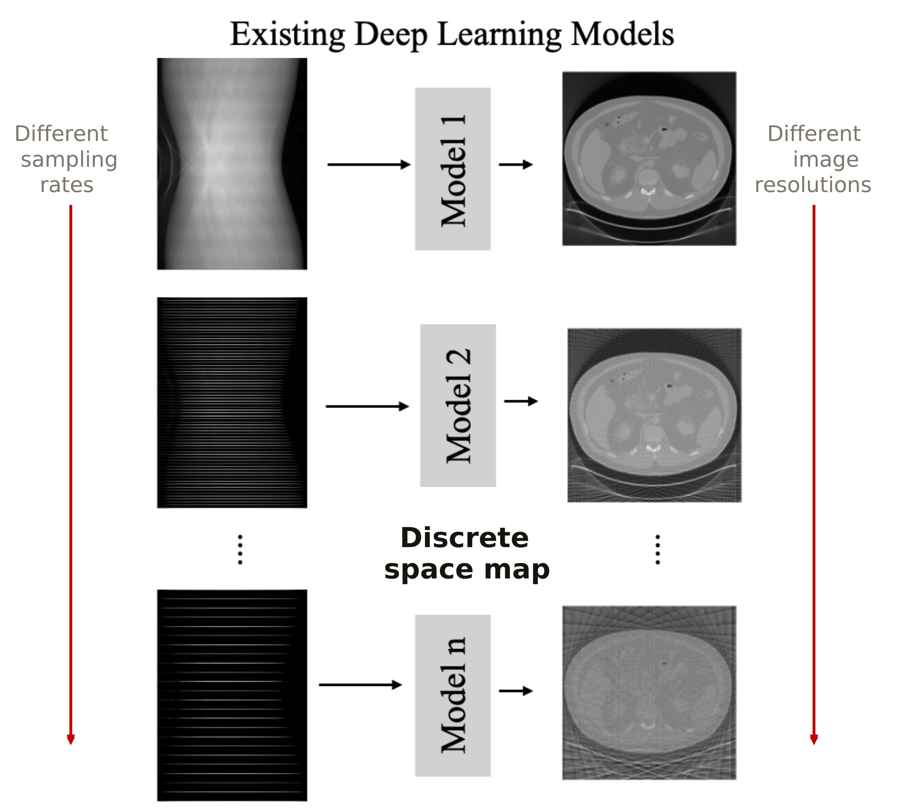
Deep learning models are very successful at learning priors that are able to recover high-quality images from sub-sampled measurements. However, each of these models is a discrete space map which is tied to one setting, i.e. one input sub-sampling rate (e.g. 18-view / 40× acceleration) and one output image resolution (e.g. 512×512 image resolution). If we want to vary any of these, which is a common requirement in clinical settings where acquisition protocols differ across organs and diagnostic purposes, we need to train a separate model for the new setting, which is not scalable.

Existing deep learning models: one model per sampling rate — Existing deep learning models: a separate model is trained for each sampling rate and output image resolution.

As an example, in the table below we show that models that are trained on 72-view sinograms don't perform well on 36-view and 18-view sinograms.

Trained model + setting	18-view test	36-view test	72-view test
LEARN — 72 views only	4.2	22.4	32.3
RegFormer — 72 views only	5.0	24.6	35.1

PSNR (dB) on the AAPM abdomen dataset. A model trained on one setting does not generalize well to another setting.

Our Proposal

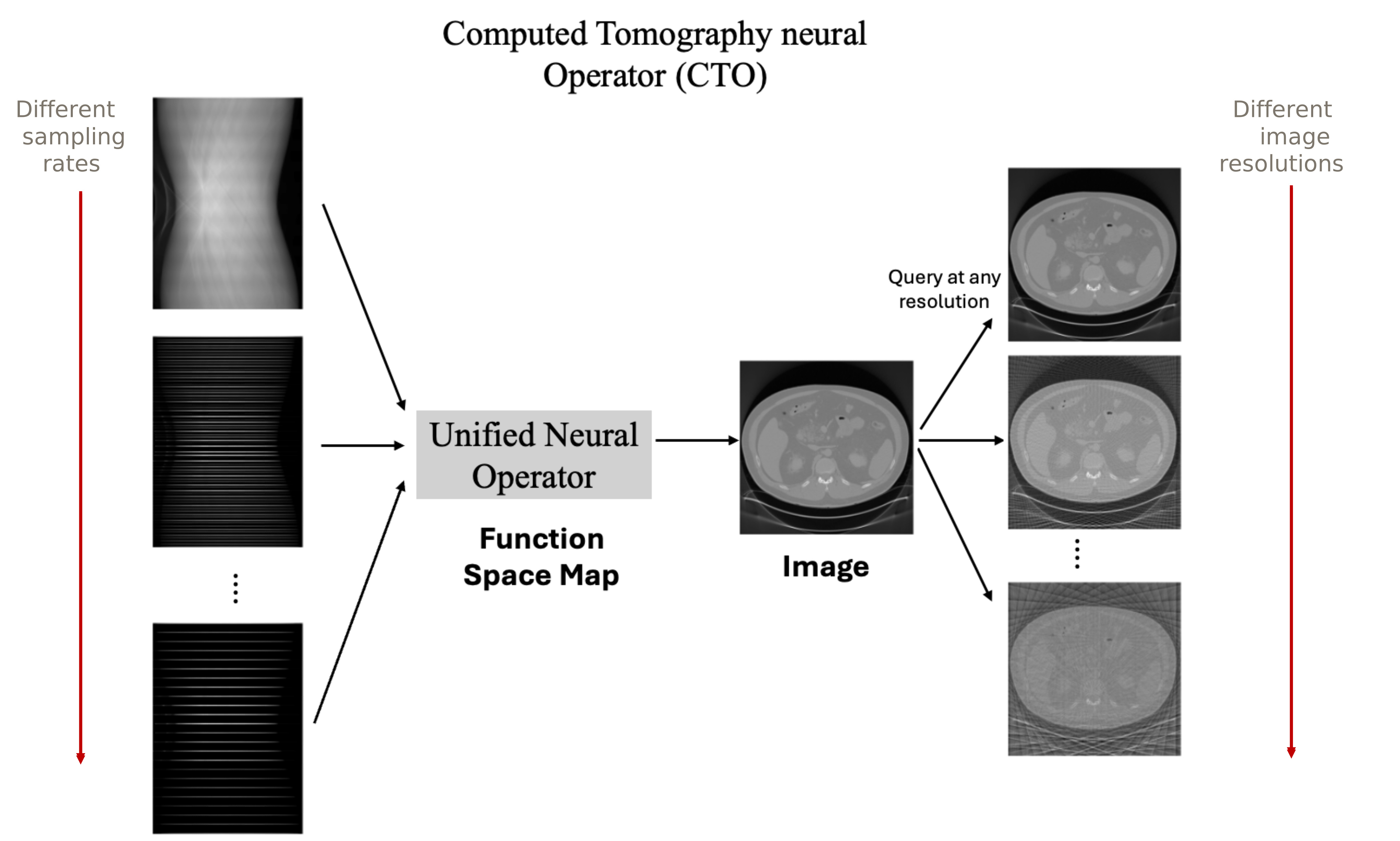
We propose that instead of training a family of discrete-space networks, we train a single function space map. We do this using Neural Operators, a deep learning architecture that learns mappings between function spaces. Since a function has infinite resolution, it can handle inputs and outputs at any arbitrary discretization or resolution. Therefore, a single neural operator can ingest sinograms at any sub-sampling rate and output reconstructed images at any image resolution without any retraining required.

A single unified neural operator across all sampling rates — A single function space map: one neural operator for all sampling rates and output resolutions.

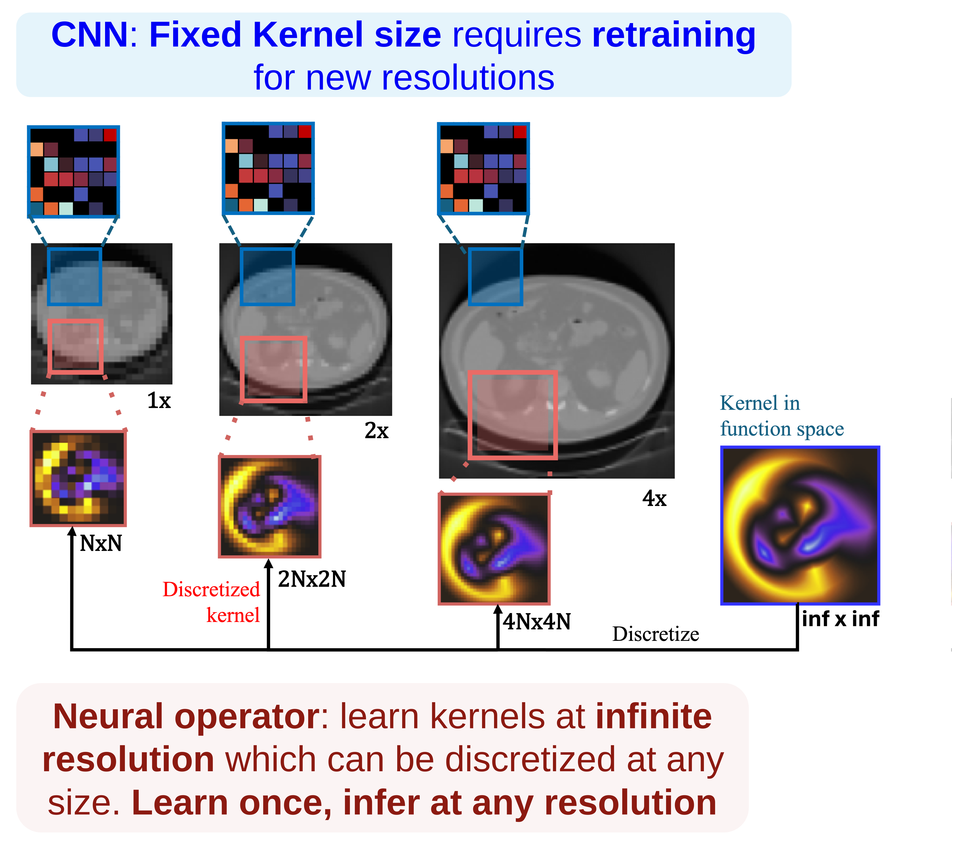
We use the Discrete–Continuous (DISCO) Neural Operator, which is a function space generalization of a traditional Convolutional Neural Network (CNN). Take a 3×3 CNN kernel for example. It has nine basis functions (which are the nine one-hot matrices), and we learn weights for each of these basis functions during training. For a DISCO convolutional kernel, the basis functions are continuous 2-D functions, and training learns the weights of these continuous functions. The final kernel is thus a weighted sum of continuous functions, and is hence a continuous function itself.

Since the final kernel is continuous, it can be discretized for any resolution such that its receptive field covers the same physical area of the image. For instance, the continuous kernel can be discretized to a 3×3 discrete kernel when working on 256×256 images and to a 6×6 kernel while working with 512×512 images. On the other hand, since CNNs have a fixed discretization, their receptive field covers a different physical area for images with different resolutions, and hence they need to be retrained for each resolution. Thus, by using DISCO neural operators, we can learn at one resolution and infer at any other resolution.

DISCO continuous kernels versus fixed CNN kernels — An example of how a continuous kernel is discretized at different resolutions.

We use the U-shaped DISCO Neural Operator (UDNO) as the building block of our architecture. It closely follows the shape and architecture of a U-Net, except that every CNN layer is replaced with a DISCO layer.

Our method: Computed Tomography neural Operator

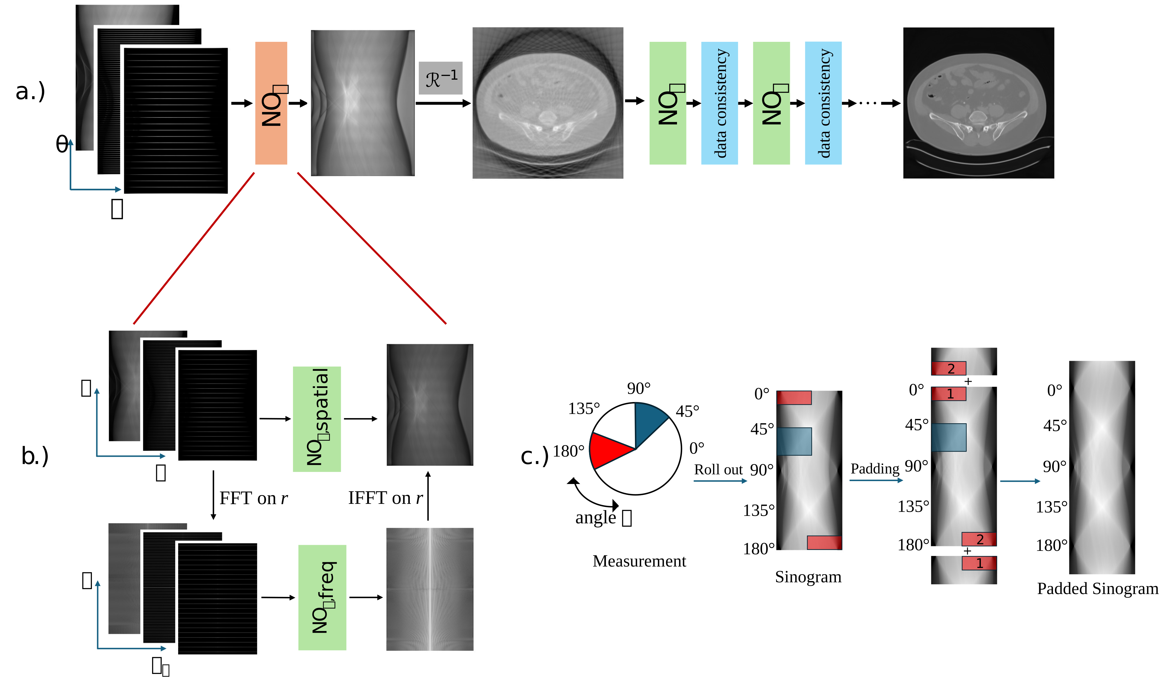
CTO architecture — a) Architecture of Computed Tomography neural Operator (CTO): sinogram-space operator $\mathrm{NO}_s$, inverse Radon transform $\mathcal{R}^{-1}$, then unrolled cascades of image-space operator $\mathrm{NO}_i$ with data consistency. b) Inside $\mathrm{NO}_s$: parallel spatial and frequency branches. c) Example of padding used in $\mathrm{NO}_s$.

Computed Tomography neural Operator, or CTO, is a dual domain neural operator. The sub-sampled sinogram (which can be sub-sampled to any rate) first gets fed into a sinogram-space neural operator $\mathrm{NO}_s$, which fills in missing information in the sinogram. Then, we pass this inpainted sinogram through an inverse Radon transform, which gives us the initial image reconstruction. This initial reconstruction is then passed through multiple cascades of image-space neural operators (labelled $\mathrm{NO}_i$ in the figure) followed by a data-consistency step. Each cascade progressively refines the image until finally we get the final reconstructed image, which is the output of CTO. In our work, we use three cascades of $\mathrm{NO}_i$ in the unrolled image-space network.

As shown in the figure, the sinogram-space neural operator $\mathrm{NO}_s$ consists of two parallel branches. The first branch operates in the spatial domain of the sinogram, thus embedding local inductive bias in the spatial domain and learning patterns directly in the native polar coordinates of the sinogram.

For the other branch, we first perform a Fourier transform along the detector axis of the sinogram. By the Fourier slice theorem,

$\mathcal{F}_r\{\mathbf{p}(\theta, r)\}(\omega) = \hat{f}(\omega\cos\theta,\ \omega\sin\theta),$

this gives us the object's 2-D frequency map in polar coordinates. As a result, the frequency branch of $\mathrm{NO}_s$ learns local patterns in the frequency domain, which correspond to global patterns in the spatial domain. The frequency branch can also be seen as a learned generalization of the ramp filter used in Filtered Back-Projection. This two-branch design ensures that we learn both local and global features, leading to better reconstruction quality.

We also design our sinogram-space neural operator to be rotationally equivariant. CT measurement is inherently rotationally equivariant. The top and bottom of the sinogram are continuous except for a left–right flip along the detector axis, so the top left of a sinogram and the bottom right of the sinogram are continuous, and vice versa.

We incorporate this symmetry in the padding we use for $\mathrm{NO}_s$. Along the $\theta$ axis, we wrap the top part of the sinogram with the bottom part, flipped along the detector axis $r$, and we also do the same for the bottom. This ensures that the network sees a continuous and physically consistent sinogram with no discontinuity in the edges, and can learn more accurate patterns. An example of the padding used in $\mathrm{NO}_s$ is shown in panel (c) above.

$\mathrm{NO}_{s,\text{freq}}$, $\mathrm{NO}_{s,\text{spatial}}$ and each $\mathrm{NO}_i$ cascade are all UDNOs.

Experiments

Multi-rate Reconstruction

For all methods, we train a single model for all sub-sampling rates, and this helps improve generalization across different rates. Training data consists of an equal number of 9-view, 18-view, 36-view and 72-view sub-sampled sinograms. We observe that CTO outperforms all baseline methods. Results are in the table below.

Category	Method	Test rate (PSNR in dB)
Category	Method	18-view	36-view	72-view
Learning-free	FBP	13.14	13.36	13.82
Learning-free	SART	24.97	25.91	26.66
Diffusion	DPS	25.68	29.13	31.64
Diffusion	ALD	25.78	28.33	30.56
Single pass	DuDoTrans	25.36	29.88	32.35
	GloReDi	29.47	31.74	32.96
	MDPRNet	25.38	27.91	30.87
Unrolled	Learned PD	25.35	27.13	29.96
	LEARN	25.51	27.53	29.90
	RegFormer	25.67	28.00	30.43
	Unrolled CNN	29.14	31.76	33.35
	CTO (ours)	31.57	35.06	37.88

Higher is better. PSNR (dB) on the AAPM Low-Dose CT dataset.

Example Reconstructions

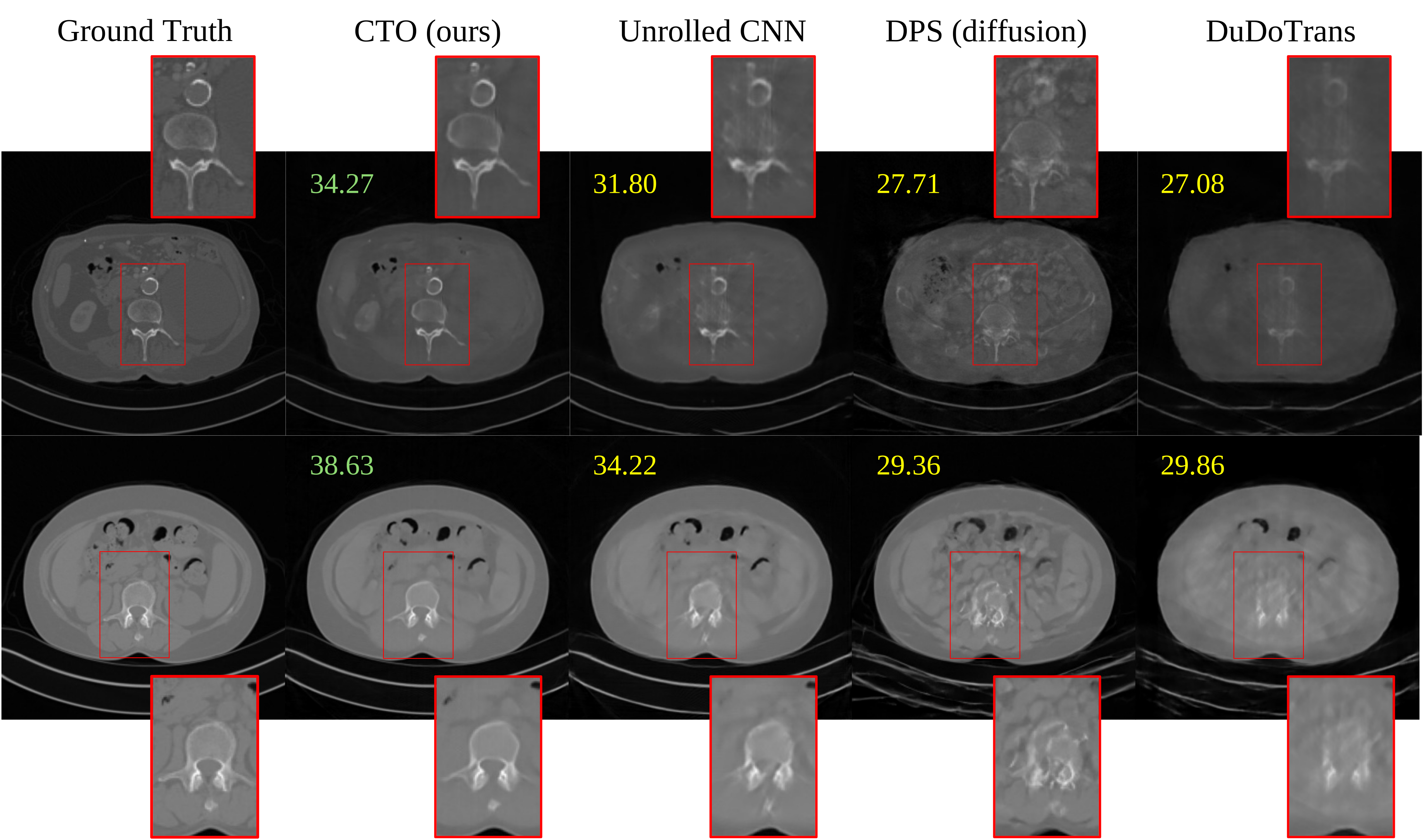
In the figure below, we present some example reconstructions from different models. In the enlarged regions you can see that CTO produces more faithful reconstructions and preserves noticeably more detail than the other methods.

Reconstructions on AAPM and kidney datasets — Example reconstructions from AAPM low-dose CT dataset (top row) and C4KC-KiTS kidney dataset (bottom row), with PSNR in the top-left corner of each image.

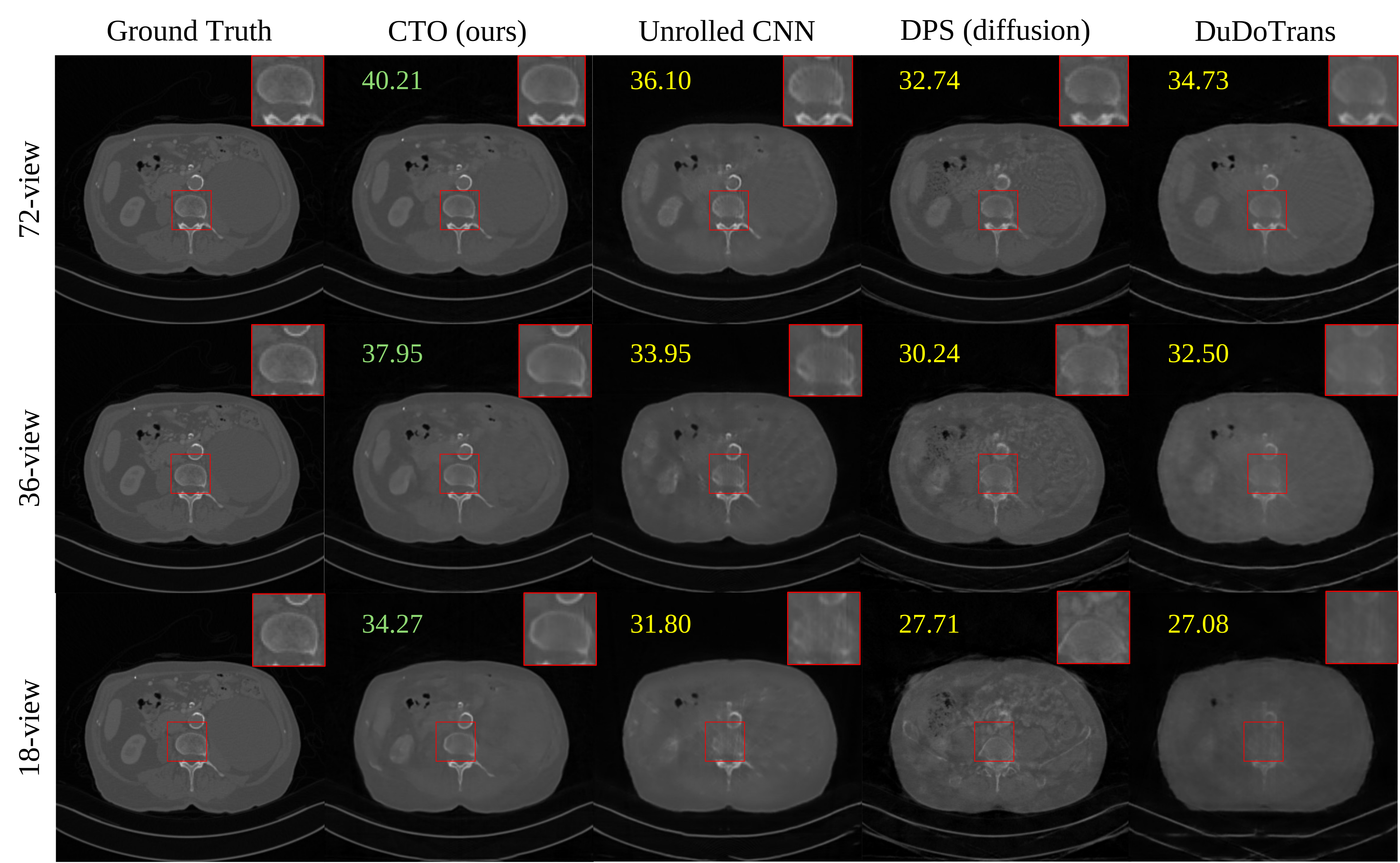
We also see that CTO holds its advantage across down-sampling rates. If you look at the enlarged regions and compare them across rates, the loss of detail as we sample less is noticeably smaller for CTO than other methods.

Reconstructions across 72-, 36- and 18-view sampling rates — The same slice reconstructed at 72-view, 36-view and 18-view sub-sampling rates using different methods.

Zero-shot super-resolution

Finally, we show that CTO also has superior zero-shot super-resolution performance, both in the image space and sinogram space.

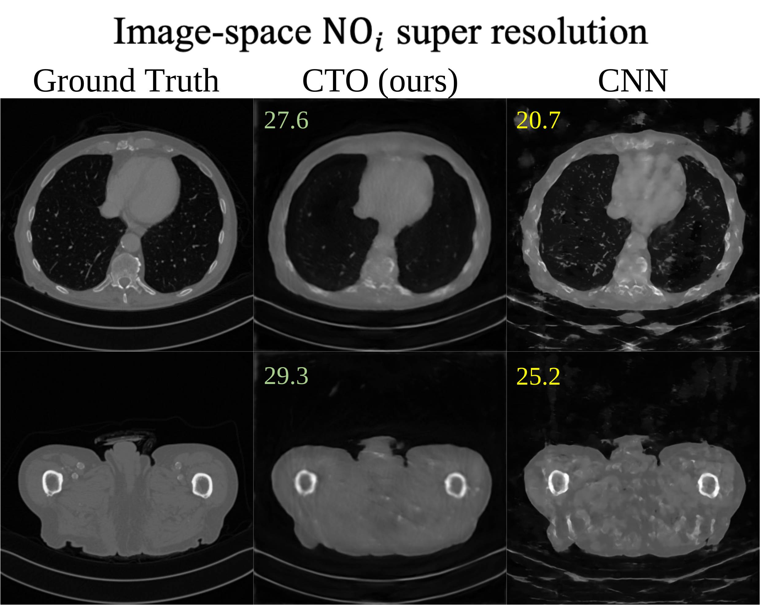
For image space, we train at 256×256 output resolution and test at 512×512 resolution with no fine-tuning. CTO performs 3 dB PSNR better than Unrolled CNN Variational Network and 4.8 dB PSNR over LEARN. As we can see in the figure, CTO also has much better reconstruction quality.

Image-space zero-shot super-resolution — Image-space super resolution: trained at 256×256 output resolution, tested at 512×512 with no fine-tuning.

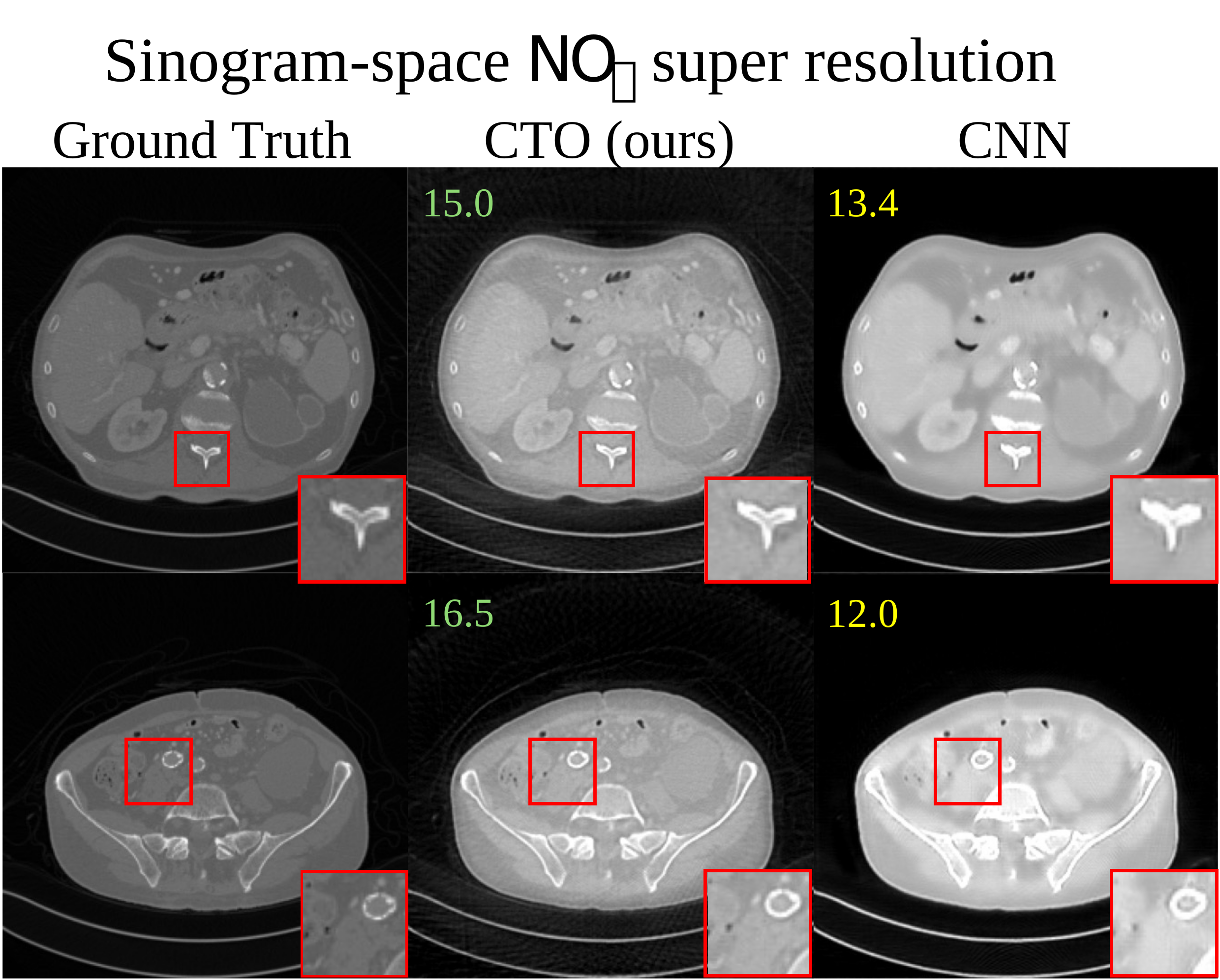
For sinogram space, if we train on a 72-view sub-sampling rate and test on a 144-view sub-sampling rate without fine-tuning, we observe that CTO performs 3.7 dB PSNR better than Unrolled CNN Variational Network, and again has better perceptual reconstruction quality.

Sinogram-space zero-shot super-resolution — Sinogram-space super resolution: trained on a 72-view sub-sampling rate, tested on 144-view with no fine-tuning.

BibTeX

@article{datta2026cto,
  author    = {Aujasvit Datta* and Jiayun Wang* and Asad Aali and Anima Anandkumar},
  title     = {Resolution-Agnostic Neural Operators for Multi-Rate Sparse-View CT},
  journal   = {arXiv preprint arXiv:2512.12236},
  abbr      = {ECCV},
  year      = {2026}
}